
More Information
Submitted: February 12, 2024 | Approved: February 26, 2024 | Published: February 27, 2024
How to cite this article: Biró L, Kozma-Bognár V, Berke J. Comparison of RGB Indices used for Vegetation Studies based on Structured Similarity Index (SSIM) J Plant Sci Phytopathol. 2024; 8: 007-012.
DOI: 10.29328/journal.jpsp.1001124
Copyright License: © 2024 Biró L, et al. This is an open access article distributed under the Creative Commons Attribution License, which permits unrestricted use, distribution, and reproduction in any medium, provided the original work is properly cited.
Keywords: Remote sensing; Unmanned aerial vehicle (UAV); Index; Structured similarity index (SSIM)

Comparison of RGB Indices used for Vegetation Studies based on Structured Similarity Index (SSIM)
Lóránt Biró1*, Veronika Kozma-Bognár2 and József Berke2
1Faculty of Commerce, Hospitality and Tourism, Budapest Business University, Hungary
2Drone Technology, and Image Processing Scientific Lab, Dennis Gabor University, Hungary
*Address for Correspondence: Lóránt Biró, Faculty of Commerce, Hospitality and Tourism, Budapest Business University, Hungary, Email: [email protected]
Remote sensing methods are receiving more and more attention during vegetation studies, thanks to the rapid development of drones. The use of indices created using different bands of the electromagnetic spectrum is currently a common practice in agriculture e.g. normalized vegetation index (NDVI), for which, in addition to the red (R), green (G) and blue (B) bands, in different infrared (IR) ranges used bands are used. In addition, there are many indices in the literature that can only be calculated from the red, green, blue (RGB) bands and are used for different purposes. The aim of our work was to objectively compare and group the RGB indices found in the literature (37 pcs) using an objective mathematical method (structured similarity index; SSIM), as a result of which we classified the individual RGB indices into groups that give the same result. To do this, we calculated the 37 RGB indexes on a test image, and then compared the resulting images in pairs using the structural similarity index method. As a result, 28 of the 37 indexes examined could be narrowed down to 7 groups - that is, the indexes belonging to the groups are the same - while the remaining 9 indexes showed no similarity with any other index.
Nowadays, with the help of drones, we can not only take detailed, high-resolution shots but also evaluate the shots using the methods used in image processing. In the present case, these represent the various filters (noise, color, edge, etc.) on the one hand, and the indices calculated from the spectrum bands on the other. The use of indices is currently common practice in agriculture; however, these indices use bands used in different infrared ranges in addition to the RGB (red, green, blue) bands. In addition, there are several indices containing only RGB bands, the most common purpose of which is to create indices formed using only RGB bands like the results of the Normalized Vegetation Index (NDVI) and Normalized Difference Red Edge Index (NDRE) indices formed using the more expensive infrared bands (Near Infrared, RedEdge).
The aim of our work is to objectively compare and group the most common RGB indices (37 pcs) currently found in the literature. Of course, it is not our goal to process all the indices that can be found in the literature, since new indices are always being created, which are usually specific to a specific plant culture. The most important question is how many groups they can be classified into, using an objective mathematical method, as well as which RGB indexes each group contains, so which indexes give almost the same result. We did not aim to examine the applicability of the indices, i.e. to what vegetation they were applied, and what is the interpretation of the results of the given index. Considering the various plant cultures, we didn't have the opportunity to do so. We wanted to use a purely mathematical method to compare the indices and draw attention to possible redundancies.
As a first step, we collected the most important RGB indices found in the literature, which are as follows (Table 1).
| Table 1: Processed RGB indices. | |||
| Index | Name | Formula | Reference |
| BCC | Blue Chromatic Coordinate Index | B/(R+G+B) | De Swaef, et al. 2021 [19] |
| BGI | Simple blue-green Ratio; Blue Green Pigment Index | B/G | Zarco-Tejada, et al. 2005 [20] |
| BI | Brightness Index | ((R2+B2+G2)/3)2 | Richardson & Wiegand 1977 [21] |
| BRVI | Blue Red Vegetation Index | (B-R)/(B+R) | De Swaef, et al. 2021 [19] |
| CIVE | Colour Index of Vegetation | 0,441r-0,881g+0,385b+18,78745 | Kataoka et al. 2003 [22] |
| ExB | Excess Blue | 1,4b-g | Mao, et al. 2003 [23] |
| ExG | Excess Green | 2g-r-b | Woebbecke, et al. 1995 [24] |
| ExGR | Excess Green-Excess Red | ExG-1,4r-g | Meyer & Neto 2008 [25] |
| ExR | Excess Red | 1,4r-g | Mao, et al. 2003 [23] |
| GCC | Green Percentage Index | G/(R+G+B) | Richardson, et al. 2007 [26] |
| GLI | Green Leaf Index | (2G-R-B)/(2G+R+B) | Louhaichi, et al. 2001 [27] |
| GR | Simple red-green Ratio | G/R | Gamon & Surfus 1999 [28] |
| GRVI | Green Red Vegetation Index | (G-R)/(G+R) | Motohka, et al. 2010 [29] |
| HI | Primary Colours Hue Index | (2*R-G-B)/(G-B) | Escadafal, et al. 1994 [30] |
| HUE | Overall Hue Index | atan(2*(B-G-R)/30,5*(G-R)) | Escadafal, et al. 1994 [30] |
| IKAW | Kawashima index | (R-B)/(R+B) | Kawashima & Nakatani 1998 [31] |
| IOR | Iron Oxide Ratio | R/B | Segal 1982 [32] |
| IPCA | Principal Component Analysis Index | 0.994*|R−B| + 0.961*|G−B| + 0.914*|G−R| | Saberioon, et al. 2014 [33] |
| MGRVI | Modified Green Red Vegetation Index | (G2-R2)/(G2+R2) | Bending, et al. 2015 [34] |
| MPRI | Modified Photochemical Reflectance Index | (G-R)/(G+R) | Yang, et al. 2008 [35] |
| MVARI | Modified Visible Atmospherically Resistant Vegetation Index | (G−B)/(G+R−B) | Yang, et al. 2008 [35] |
| NDI | Normalized Difference Index | 128*(((G-R)/(G+R))+1) | Mcnairn & Protz 1993 [36] |
| NGBDI | Normalized Green Blue Difference Index | (G-B)/(G+B) | Du & Noguchi 2017 [37] |
| NGRDI | Normalized Green Red Difference Index | (G-R)/(G+R) | Gitelson, et al. 2002 [38] |
| RCC | Red Chromatic Coordinate Index | R/(R+G+B) | De Swaef et al. 2021 [19] |
| RGBVI | Red Green Blue Vegetation Index | (G2-(B*R))/(G2+(B*R)) | Bending, et al. 2015 [34] |
| PRI | Photochemical Reflectance Index | R/G | Gamon, et al. 1997 [39] |
| SAVI | Soil Adjusted Vegetation Index | (1,5*(G-R))/(G+R+0,5) | Li, et al. 2010 [40] |
| SCI | Soil Colour Index | (R-G)/(R+G) | Mathieu, et al. 1998 [41] |
| SI | Spectral Slope Saturation Index | (R-B)/(R+B) | Escadafal, et al. 1994 [30] |
| TGI | Triangular Greenness Index | G-0,39*R-0,61*B | Hunt, et al. 2013 [42] |
| VARI | Visible Atmospherically Resistant Vegetation Index | (G-R)/(G+R-B) | Gitelson, et al. 2002 [38] |
| VDVI | Visible Band-Difference Vegetation Index | (2G-R-B)/(2G+R+B) | Wang, et al. 2015 [43] |
| VEG | Vegetative Index | G/(R0,667*B0,334) | Hague, et al. 2006 [44] |
| VIgreen | Vegetation Index Green | (G-R)/(G+R) | Gitelson, et al. 2002 [38] |
| vNDVI | Visible NDVI | 0,5268*(r-0,1294*g0,3389*b-0,3118) | Costa, et al. 2020 [13] |
| WI | Woebbecke Index | (G-B)/(R-G) | Woebbecke, et al. 1995 [24] |
| R: Red Band; G: Green Band; B: Blue Band; r: R/(R+G+B); g: G/(R+G+B); b: G/(R+G+B). | |||
The test image used for the RGB indices (Figure 1) was taken in JPG picture file format with a DJI Mavic Mini rotary-wing quadcopter drone, in Vértes mountains, Hungary. The recording shows low and higher vegetation, shade, a barren dirt road, and white limestone piles, so the recording provides a good opportunity to test the indices. The parameters of the camera used for recording are as follows. Sensor type 1/2.3" CMOS (Complementary Metal-Oxide Semiconductor sensor), effective pixel 12 Megabyte, image size 4000 x 3000 pixels, viewing angle 83°, focal length 24 mm and aperture f/2.8.
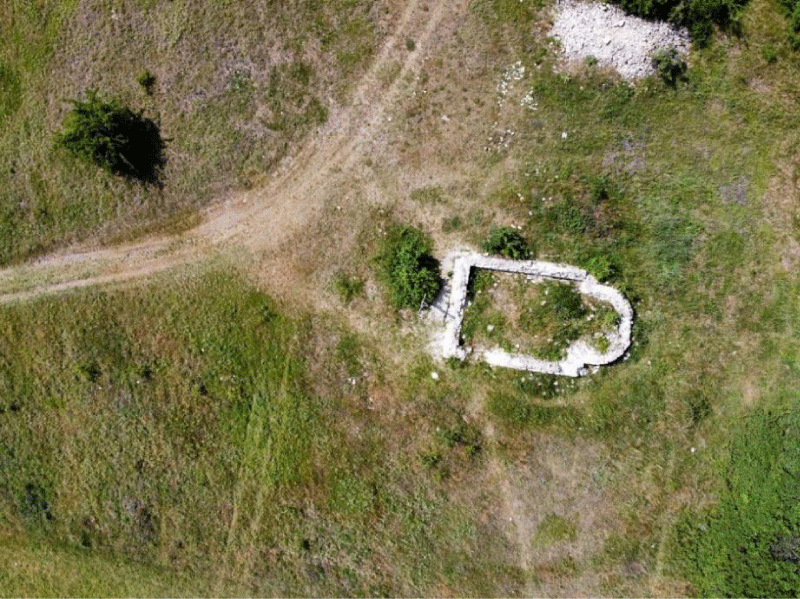
Figure 1: Test image used for RGB indices.
To find out which band carries the most information, we calculated the Shannon’s entropy of each band [1,2] (Table 2).
| Table 2: Information content and self-similar spectral fractal dimension of the bands of the test image. | |||||||
| Band | (S)FD, S [bit] | Number of unique pixels | SFD DSR Number (8-bit) | SFD DSR Number (16-bit) | SFD DSR Number (real bit) | EW-SFD DSR Number (real bit - valuable containing) | Entropy |
| Red | 8 | 256 | 1 | 0,8314 | 1,0000 | 0,9652 | 7,6156 |
| Green | 8 | 256 | 1 | 0,8314 | 1,0000 | 0,9479 | 7,4693 |
| Blue | 8 | 256 | 1 | 0,8314 | 1,0000 | 0,8660 | 7,4777 |
| Red, Green | 8 | 18908 | 1,7510 | 1,4641 | 1,7510 | 1,5675 | 13,0449 |
| Red, Green, Blue | 8 | 270561 | 2,4699 | 1,9826 | 2,4699 | 2,2178 | 16,5068 |
So, those indexes that contain the band with the highest entropy give the right result (differentiate the vegetation sufficiently [3,4].
Table 2 contains the values calculated according to the reference [5,6] for the self-similar (Spectral Fractal Dimension) image structure. All of this is important for higher-order image processing processes, information security analysis [3,7,8], and for the investigation of the effect of image sensor noise on the image structure [9,10].
From the RGB bands of the recording shown in Figure 1, we calculated the individual indices with the Quantum GIS (QGIS) software based on the formulas shown in Table 1, and then each index image was created in two file formats. As a first step, we created a "false color" image; with the same colour scale for each index, where the red color represents the negative or 0 value, while the blue color represents the more positive values. This way you can easily compare the completed index images. As a second step, the index image was saved as a grayscale image since the mathematical method for objective comparison only handles grayscale JPG images.
The pairwise comparison of the index images was done based on the structural similarity index [11], which results in a value between -1 and +1, where -1 represents the complete difference between the two images, while + 1 for a complete match. The comparisons were made in the Python Programming Language with the "scikit-image" program package, which also includes the SSIM method [12].
As a result of the comparisons, we obtained a similarity matrix, which gives the pairwise similarity value of each index. We considered only indices with a pairwise SSIM value ≥ 0.9 to be the same. Based on the values of the similarity matrix, the following indices show complete agreement (the formulas are the same, so SSIM = 1):
- ExG = GCC (for the exact name of the indexes see Table 1.)
- GLI = VDVI
- GRVI = MPRI, NDI, NGRDI, VIgreen (of course these indices are also the same)
- IKAW = SI
During the examination of further similarities, we obtained 7 groups (Table 3) in which the SSIM value of the indices is 1.0 > x ≥ 0.9.
| Table 3: Groups of similar indices (SSIM 1.0 > x ≥ 0.9). | ||||||
| 1. Group | 2. Group | 3. Group | 4. Group | 5. Group | 6. Group | 7. Group |
| GRVI | BCC | CIVE | HI | GLI | IOR | IPCA |
| ExGR | BRVI | ExG | MVARI | VDVI | VEG | TGI |
| ExR | IKAW | GCC | ||||
| MGRVI | NGBDI | |||||
| MPRI | RGBVI | |||||
| NDI | SI | |||||
| NGRDI | ||||||
| SAVI | ||||||
| SCI | ||||||
| VARI | ||||||
| VIgreen | ||||||
Out of the 37 indexes, 28 indexes are included in the above 7 groups. From these groups, we selected one characteristic index that best characterizes the given group (by visual comparison), these are MGRVI, RGBVI, GCC, MVARI, GLI, VEG, and TGI. The remaining 9 indices can be considered unique, i.e. not like any other index, they are: BGI, BI, ExB, GR, HUE, RCC, PRI, vNDVI, and WI.
Thus, as a result, the 38 indexes can be considered a total of 16 different indexes, which are as follows: BGI, BI, ExB, GCC, GLI, GR, HUE, MGRVI, MVARI, RCC, RGBVI, RGI (same as PRI), TGI, VEG, vNDVI, WI (Figure 2).
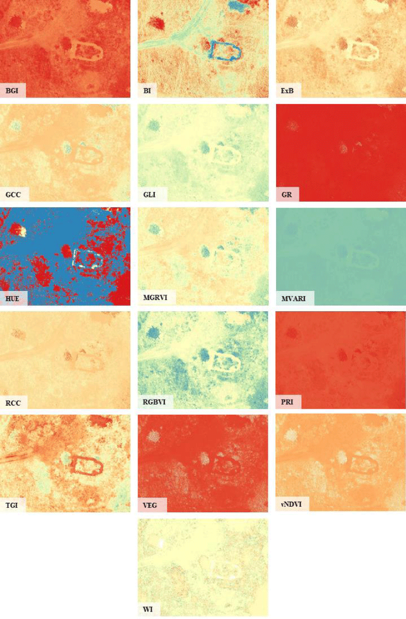
Figure 2: Individual indices obtained as a result of comparison.
Based on the examination of the most common 37 RGB indices found in the literature using the objective similarity method, we can therefore speak of 16 independent indices. It is important to emphasize that this does not mean that redundant indexes are unnecessary, but only that during image data processing, we can even use several indexes to answer a question, which will probably give a similar result. During the comparisons, we ignored the original applicability of the given indices, that is, on what type of vegetation they were first used. However, when solving the given problem, this aspect must also be considered before the index is selected.
Further investigation can be performed on several types of vegetation and the 16 types of indices can be interpreted. But perhaps the most important question is which index gives the most similar results to the NDVI index, as this could reduce the use of multispectral cameras during vegetation surveys with unmanned aerial vehicles (UAVs).
So far, we have not found works of a similar nature and purpose in the literature that is, where indexes were compared using an objective statistical method. The comparison of the vegetation indices was only aimed at which RGB indices give similar results as the multispectral (MS) indices, tested on a specific type of vegetation [13-18]. The present work does not examine the similarity of the RGB and MS indices on a specific vegetation, but independently of the vegetation, namely in an objective statistical manner. Thus, the results are most likely true for most vegetation.
Future developments include the creation of an open image database suitable for the presented SSIM-based comparative studies based on various aspects (UAVs, recording parameters, image sensor devices and types, image file formats, vegetation types, and vegetation periods). Thus, based on the various aspects above, we will be able to objectively compare the pictures. Hopefully, we will be able to report on their results soon.
Project no. TKP2021-NVA-05 has been implemented with the support provided by the Ministry of Innovation and Technology of Hungary from the National Research, Development and Innovation Fund, financed under the TKP 2021 funding scheme.
- Shannon CEA. A mathematical theory of communication. The Bell System Technical Journal. 1948; 27: 379-423; 623-656.
- Rényi A. On measures of entropy and information. Proceedings of the 4th Berkeley Symposium on Mathematics, Statistics, and Probability. 1961; 4:1; 547-561.
- Kozma-Bognár V, Berke J. New Applied Techniques in Evaluation of Hyperspectral Data. Georgikon for Agriculture. 2009; 12: 25-48.
- Kozma-Bognar V, Berke J. New Evaluation Techniques of Hyperspectral Data. J. of Systemics, Cybernetics and Informatics. 2010; 8: 49-53.
- Berke J. Measuring of spectral fractal dimension. New Math. Nat. Comput. 2007; 3: 409-418, doi: https://doi.org/10.1142/S1793005707000872 .
- Berke J, Gulyás I, Bognár Z, Berke D, Enyedi A, Kozma-Bognár V, Mauchart P, Nagy B, Várnagy Á, Kovács K, Bódis J. Unique algorithm for the evaluation of embryo photon emission and viability, preprint. 2024.
- Berke J. Using spectral fractal dimension in image classification. In: Sobh, T. (ed.), Innovations and Advances in Computer Sciences and Engineering. 2010; 237-242. Springer Dordrecht. https://doi.org/10.1007/978-90-481-3658-2.
- Karydas CG. Unified scale theorem: a mathematical formulation of scale in the frame of Earth observation image classification. Fractal Fract. 2021; 5: 127. https://doi.org/10.3390/fractalfract5030127.
- Rosenberg E. Fractal Dimensions of Networks. Springer Nature Switzerland AG. 2020.
- Dachraoui C, Mouelhi A, Drissi C, Labidi S. Chaos theory for prognostic purposes in multiple sclerosis. Transactions of the Institute of Measurement and Control. 2021; 11. https://doi.org/10.1177/01423312211040309.
- Wang Z, Bovik AC, Sheikh HR, Simoncelli EP. Image quality assessment: from error visibility to structural similarity. IEEE Trans Image Process. 2004 Apr;13(4):600-12. doi: 10.1109/tip.2003.819861. PMID: 15376593.
- van der Walt S, Schönberger JL, Nunez-Iglesias J, Boulogne F, Warner JD, Yager N, Gouillart E, Yu T; scikit-image contributors. scikit-image: image processing in Python. PeerJ. 2014 Jun 19;2:e453. doi: 10.7717/peerj.453. PMID: 25024921; PMCID: PMC4081273.
- Costa L, de Morais NL, Ampatzidis Y. A new visible band index (vNDVI) for estimating NDVI values on RGB images utilizing genetic algorithms. Computers and Electronics in Agriculture. 2020; 172. https://doi.org/105334. 10.1016/j.compag.2020.105334.
- Feng H, Tao H, Li Z, Yang G, Zhao C. Comparison of UAV RGB Imagery and Hyperspectral Remote-Sensing Data for Monitoring Winter Wheat Growth. Remote Sensing. 2022; 14: 3811. https://doi.org/10.3390/rs14153811 .
- Fuentes-Peñailillo F, Ortega-Farias S, Rivera M, Bardeen M, Moreno M. Comparison of vegetation indices acquired from RGB and Multispectral sensors placed on UAV. ICA-ACCA 2018, October 17-19, 2018, Greater Concepci´on, Chile. 2019.
- Furukawa F, Laneng LA, Ando H, Yoshimura N, Kaneko M, Morimoto J. Comparison of RGB and Multispectral Unmanned Aerial Vehicle for Monitoring Vegetation Coverage Changes on a Landslide Area. Drones. 2021; 5: 97. https://doi.org/10.3390/drones5030097.
- Gracia-Romero A, Kefauver SC, Vergara-Díaz O, Zaman-Allah MA, Prasanna BM, Cairns JE, Araus JL. Comparative Performance of Ground vs. Aerially Assessed RGB and Multispectral Indices for Early-Growth Evaluation of Maize Performance under Phosphorus Fertilization. Front Plant Sci. 2017 Nov 27;8:2004. doi: 10.3389/fpls.2017.02004. PMID: 29230230; PMCID: PMC5711853.
- Yuan Y, Wang X, Shi M, Wang P. Performance comparison of RGB and multispectral vegetation indices based on machine learning for estimating Hopea hainanensis SPAD values under different shade conditions. Front Plant Sci. 2022 Jul 22;13:928953. doi: 10.3389/fpls.2022.928953. PMID: 35937316; PMCID: PMC9355326.
- De Swaef T, Maes WH, Aper J, Baert J, Cougnon M, Reheul D, Steppe K, Roldán-Ruiz I, Lootens P. Applying RGB- and Thermal-Based Vegetation Indices from UAVs for High-Throughput Field Phenotyping of Drought Tolerance in Forage Grasses. Remote Sensing. 2021; 13(1): 147. https://doi.org/10.3390/rs13010147 .
- Zarco-Tejada PJ, Berjón A, López-Lozano R, Miller JR, Martín P, Cachorro V, González MR, de Frutos A. Assessing vineyard condition with hyperspectral indices: Leaf and canopy reflectance simulation in a row-structured discontinuous canopy. Remote Sensing of Environment. 2005; 99(3): 271-287. https://doi.org/10.1016/j.rse.2005.09.002.
- Richardson AJ, Wiegand C. Distinguishing Vegetation from Soil Background Information. Photogrammetric Engineering and Remote Sensing. 1977; 43: 1541-1552.
- Kataoka T, Kaneko T, Okamoto H, Hata S. Crop growth estimation system using machine vision. In: IEEE/ASME International Conference on Advanced Intelligent Mechatronics, 2003, Kobe. Proceedings. Piscataway: IEEE. 2003; 2:1; 1079-1083.
- Mao W, Wang Y, Wang Y. Real-time detection of between row weeds using machine vision. ASABE Annual Meeting. Las Vegas, NV. 2003.
- Woebbecke DM, Meyer GE, Bargen KVON, Mortensen DA. Color indices for weed identification under various soil, residue, and lighting conditions. Transactions of the ASAE, Michigan. 1995; 38: 1; 259-269.
- Meyer GE, Camargo Neto J. Verification of color vegetation indices for automated crop imaging applications. Computers and Electronics in Agriculture. Athens. 2008; 63: 2; 282-293.
- Richardson AD, Jenkins JP, Braswell BH, Hollinger DY, Ollinger SV, Smith ML. Use of digital webcam images to track spring green-up in a deciduous broadleaf forest. Oecologia. 2007 May;152(2):323-34. doi: 10.1007/s00442-006-0657-z. Epub 2007 Mar 7. PMID: 17342508.
- Louhaichi M, Borman MM, Johnson DE. Spatially Located Platform and Aerial Photography for Documentation of Grazing Impacts on Wheat. Geocarto International. 2001; 16:1; 65-70. DOI: 10.1080/10106040108542184.
- Gamon JA, Surfus JS. Assessing leaf pigment content and activity with a reflectometer. New Phytologist. 1999; 143:105-117. https://doi.org/10.1046/j.1469-8137.1999.00424.x.
- Motohka T, Nasahara KN, Oguma H, Tsuchida S. Applicability of green-red vegetation index for remote sensing of vegetation phenology. Remote Sensing, Amsterdam. 2010; 2: 10; 2369-2387.
- 30. Escadafal R, Belghit A, Ben-Moussa A. Indices spectraux pour la télédétection de la dégradation des milieux naturels en Tunisie aride. In: Guyot, G. réd., Actes du 6eme Symposium international sur les mesures physiques et signatures en télédétection, Val d’Isère (France), 17-24 Janvier. 1994; 253-259.
- Kawashima S, Nakatani M. An Algorithm for Estimating Chlorophyll Content in Leaves Using a Video Camera. Annals of Botany. 1998; 81(1):49-54. https://doi.org/10.1006/anbo.1997.0544 .
- Segal D. Theoretical Basis for Differentiation of Ferric-Iron Bearing Minerals, Using Landsat MSS Data. Proceedings of Symposium for Remote Sensing of Environment, 2nd Thematic Conference on Remote Sensing for Exploratory Geology. Fort Worth, TX. 1982; 949-951.
- Saberioon MM, Amin MSM, Anuar AR, Gholizadeh A, Wayayok A, Khairunniza-Bejo S. Assessment of rice leaf chlorophyll content using visible bands at different growth stages at both the leaf and canopy scale. International Journal of Applied Earth Observation and Geoinformation, Amsterdam. 2014; 32: 35-45.
- Bendig J, Yu K, Aasen H, Bolten A, Bennertz S, Broscheit J, Gnyp ML, Bareth G. Combining UAV-based plant height from crop surface models, visible, and near infrared vegetation indices for biomass monitoring in barley. International Journal of Applied Earth Observation and Geoinformation. Amsterdam. 2015; 39: 79-87.
- Yang Z, Willis P, Mueller R. Impact of band-ratio enhanced AWIFS image to crop classification accuracy. Pecora. 2008; 17:18-20.
- McNairn H, Protz R. Mapping Corn Field Residue Cover on Agricultural Fields in Oxford County, Ontario, Using Thematic Ma. Canadian Journal of Remote Sensing. 2014; 19.
- Du M, Noguchi N. Monitoring of Wheat Growth Status and Mapping of Wheat Yield’s within-Field Spatial Variations Using Color Images Acquired from UAV-camera System. Remote Sensing. 2017; 9(3):289. https://doi.org/10.3390/rs9030289 .
- Gitelson A, Kaufman Y, Rundquist D. Novel Algorithms for Remote Estimation of Vegetation Fraction. Remote Sensing of Environment. 2002; 80: 76-87. https://doi.org/10.1016/S0034-4257(01)00289-9.
- Gamon JA, Serrano L, Surfus JS. The photochemical reflectance index: an optical indicator of photosynthetic radiation use efficiency across species, functional types, and nutrient levels. Oecologia. 1997 Nov;112(4):492-501. doi: 10.1007/s004420050337. PMID: 28307626.
- Li Y, Chen D, Walker CN, Angus JF. Estimating the nitrogen status of crops using a digital camera. Field Crops Research, Amsterdam. 2010; 118:3; 221-227.
- Mathieu R, Pouget M. Relationships between satellite-based radiometric indices simulated using laboratory reflectance data and typic soil colour of an arid environment. Remote Sensing of Environment. 1998; 66:17-28.
- Hunt ER Jr., Doraiswamy PC, McMurtrey JE, Daughtry CST, Perry EM, Akhmedov B. A visible band index for remote sensing leaf chlorophyll content at the canopy scale. Publications from USDA-ARS / UNL Faculty. 2013; 1156.
- Wang X, Wang M, Wang S, Wu Y. Extraction of vegetation information from visible unmanned aerial vehicle images. Nongye Gongcheng Xuebao/Transactions of the Chinese Society of Agricultural Engineering. 2015; 31:5; 152-159.
- Hague T, Tillett ND, Wheeler H. Automated crop and weed monitoring in widely spaced cereals. Precision Agriculture, Berlin. 2006; 7:1; 21-32.