
More Information
Submitted: 24 September 2019 | Approved: 03 October 2019 | Published: 04 October 2019
How to cite this article: Kerr RA, Zhebentyayeva T, Saski C, McCarty LB. Comprehensive phenotypic characterization and genetic distinction of distinct goosegrass (Eleusine indica L. Gaertn.) ecotypes. J Plant Sci Phytopathol. 2019; 3: 095-100.
DOI: 10.29328/journal.jpsp.1001038
Copyright License: © 2019 Kerr RA, et al. This is an open access article distributed under the Creative Commons Attribution License, which permits unrestricted use, distribution, and reproduction in any medium, provided the original work is properly cited.
Keywords: Eleusine indica L. Gaertn.; Turfgrass; Weed control

Comprehensive phenotypic characterization and genetic distinction of distinct goosegrass (Eleusine indica L. Gaertn.) ecotypes
Robert A Kerr1*, Tatyana Zhebentyayeva2, Christopher Saski1 and Lambert B McCarty1
1Department of Plant and Environmental Sciences, Clemson University, 130 McGinty Court, Clemson, SC 29634, USA
2The Schatz Center for Tree Molecular Genetics, Department of Ecosystem Science and Management, The Pennsylvania State University, University Park, PA, USA
*Address for Correspondence: Robert A Kerr, Department of Plant and Environmental Sciences, Clemson University, 130 McGinty Court, Clemson, USA, Tel: 312 519 7940; Email: [email protected]
Goosegrass (Eleusine indica L. Gaertn.) is a troublesome weed in turfgrass systems throughout the world. The development of herbicide resistant ecotypes has occurred to multiple modes of action. Goosegrass is a prolific seed producer (~50,000 per plant), fast growing and diverse weed. Such growing attributes make it essential to have a better understanding of the genetic diversity of various ecotypes. The objectives of this study were to determine if morphologically distinct goosegrass ecotypes collected in Florida were phenotypically distinct and genetically different. Phenotypically, the goosegrass ecotypes can be classified as follows; dwarf, intermediate 1 (int_I), intermediate 2 (int_II) and wild. The dwarf had the least seedheads followed by the wild ecotype; 5 and 17 respectively, while int_I and int_II had highest number of seedheads; 22 and 34 respectively. The dwarf ecotype had lowest height of 6 cm and the wild ecotype had highest height of 36 cm. Dwarf and int_II ecotypes had shortest internode length of 0.2 cm and 1 cm, respectively, while the wild ecotype had longest internode length of 7 cm. The dwarf ecotype had lowest number of racemes per plant of 1, while the wild ecotype had highest number of racemes per plant of 7. Total biomass was lowest for the dwarf and int_II ecotype; 0.7 g and 1.5 g, respectively, and total biomass was highest for the wild ecotype at 5 g. Gene sequencing of two rice (Oryza) gene sequences (accession AP014964 (gene A) and AP014965 (gene B)) and subsequent phylogenetic analysis suggest the ecotypes are genetically different. Three single nucleotide polymorphisms (SNP) of interest were discovered indicating allelic differences between ecotypes.
Invasive and/or weed species often acclimate readily to different environmental conditions. One mechanism weeds utilize to survive and outcompete desirable plant species to is readily adapt to new habitats and environmental conditions [1,2].
To understand how weeds evolve to a wide ecological distribution, two alternate hypotheses are suggested; phenotype plasticity and locally adapted ecotypes [3].
Phenotypic plasticity or differences between populations is thought to be environmental-induced variations. In this scenario, the genotype of individuals within a population is plastic, therefore individuals can cope with different environments and/or habitats. Alternatively, for locally adapted ecotypes, the phenotypic variations between populations are genetically based [3]; therefore, different populations are locally adapted to the given habitat. Saidi et al., noted morphologically distinct ecotypes of goosegrass have been found throughout Malaysia [4].
Goosegrass a self-pollinating diploid is a major weed of turfgrass systems, and occurs in a number of different ecological habitats [4-6]. The development of herbicide resistant goosegrass is an example of locally adapted ecotypes [5,7]. Goosegrass has developed resistance to a number of herbicides, including: glyphosate [8], paraquat [9], metribuzin plus MSMA [10], glufosinate plus paraquat [11], and oxadiazon [12].
Goosegrass plants survive in different habitats on golf courses, ranging from highly maintained putting greens to the unmaintained natural areas [13]. Plants found in the different habitats are morphologically distinct such as populations on putting greens often exhibit a dwarf-like growth habit, while in the natural unmaintained habitat, goosegrass plants exhibit a tall growth habit [14]. One hypotheses for the development of the different ecotypes, is being able to survive the intense management practices such as low mowing height (< 3 mm) used on putting greens.
Burdon noted genetically diverse ecotypes occur within any population of weed species [15]. Genetic diversity leads to the development of diverse weed populations and ecotypes, and understanding the relationship between genetic and morphological diversity of plant ecotypes will lead to a better understanding of their adaptability [4,16,17]. Research is needed to elucidate the relationship between genetic and morphological diversity of goosegrass [4]. The objectives of this study were: 1) determine if goosegrass ecotypes collected in Florida were phenotypically distinct; and 2) determine if goosegrass ecotypes collected in Florida were genetically different.
In October 2014, seeds from a dwarf growing goosegrass ecotype were collected from a putting green at Deep Creek Golf Club, Punta Gorda, FL (27.01 °N, 82.01 °W); and seeds from a wild goosegrass ecotype growing in non-maintained rough were collected at Del Tura Golf Club, Fort Myers, FL (26.73 °N, 82.01 °W). Soil at both sites is an Immokalee (Sandy, siliceous, hyperthermic) Arenic Alaquods. The ecotype collected from the putting green was mowed at 3 mm, the height of the non-maintained rough was 300 mm. Seeds from multiple plants were collected at each location and then brought to Clemson University, Clemson, SC and stored at 4 °C.
In June 2016, seeds were sown in 1020 NCR trays (Landmark Plastic Corporation, Akron, OH, USA) filled with a sterile growing medium (Farfard® Growing Mix 3B; Sun Gro Horticulture Agawam, MA, USA). Trays were placed on a misting bench to promote germination for a period of 10 days, then relocated into a greenhouse. Once plants emerged and matured to a two-leaf stage, seedlings were transplanted to 10 cm by 9 cm greenhouse pots (Landmark Plastic Corporation, Akron, OH, USA) filled with a sterile growing medium (Farfard® Growing Mix 3B; Sun Gro Horticulture Agawam, MA, USA). The greenhouse experiment was arranged as a completely randomized design and conducted, June - September 2016, maximum and minimum temperatures were 30 °C and 23 °C, respectively. Light intensity was maintained at a minimum of 500 µmoles m-2 s-1 with a 14 h photoperiod, via supplemental lighting. Plants were sub-irrigated to prevent moisture stress. Plants were not clipped and no supplemental fertility was added for the duration of the study.
Plants were grown until the production of seedheads and leaf senescence (10 weeks), at which point the life cycle was considered complete. Six individuals exhibiting each ecotype were then selected and phenotypic data collected for the following traits; number of seedheads; plant height; internode length; raceme length; above ground biomass; and, total surface area of above ground biomass. Observations lead to the grouping of four ecotypes; dwarf, intermediate 1 (int_I), intermediate 2 (int_II), and wild. In addition, young green leaves were collected from each of the 24 individuals and lyophilized (freeze dried) for DNA extraction.
The number of seedheads present on individual plants were counted. Plant height was measured (cm) from plant crown to the top of the longest raceme or leaf. Twenty internodes on each plant and the length of twenty racemes on each plant were measured (cm) and averaged. Above ground biomass was separated from the root material at the crown then oven dried at 80 °C for 72 h to determine dry weight (DW). Prior to being oven dried, a subsample was removed to quantify the plants surface area using WinRhizo root-scanning software (Regent Instruments Inc., Ottawa, ON Canada); the subsample was oven dried separately. The surface area (SA) of the entire sample was determined by the following equation [18].
Where subsample SA is the surface area of the subsample, subsample DW is the dry weight of the subsample, and sample DW is the total dry weight of the plant.
DNA extraction
Genomic DNA was extracted from young, expanding leaf biomass using a modified CTAB-based protocol as described by Kubisiak, et al. [19]. Briefly, 50 mg of lyophilized (freeze dried) leaf tissue was added to 1 ml round bottom grinding tubes and stored at -80 °C until extraction. At extraction, 750 µl 1X extraction buffer containing 1.0 µl/ml 2-mercaptoethanol was added. One grinding bead was added per tube and samples ground in a Retsch Mixer Mix MM 400 (Retsch Lab Equipment, Haan, Germany) at 30 oscillation cycles per second for 10 minutes - afterwards plate orientation was switched and reground for another 10 minutes. Tubes were centrifuged at 6,000 rpm for 20 minutes, followed by supernatant removal. The pellet was reconstituted with 200 µl of organelle wash buffer, 4 µl RNaseA (10 mg/ml), and 80 µl 5% sarkosyl (N-Lauroyl Sarcosine); placed on a mixer mill and shaken at 30 oscillation cycles per second for 15 seconds, and then incubated at room temperature for 30 minutes. Plates were centrifuged at 6,000 rpm for 2 minutes, then 72 µl, 5 M NaCl, 80 µl CTAB/NaCl and 3 µl Proteinase K (20 mg/ml) was added. Plates were then shaken by hand to mix, and incubated at 65 °C for 15 minutes and then placed in -20 °C freezer for 2 minutes to cool. Following cooling, plates were centrifuged at 6,000 rpm for 2 minutes, then 400 µl chloroform/octanol (24:1) was added and mixed gently using the mixer mill for 30 oscillation cycles per second for a total of 15 seconds. Plates were then centrifuged at 6,000 rpm for 20 minutes, the upper aqueous phase transferred to new flat-bottomed 1 ml tubes and DNA extracted with at least 1 volume of ice cold 2-propanol, mixed gently and thoroughly. Extracts were centrifuged at 6,000 rpm for 10 minutes to pellet DNA, supernatant then gently poured off, 200 µl of 70% ethanol then added, and mixed thoroughly by hand. Plates were then centrifuged at 6,000 rpm for 5 minutes to re-pellet DNA, 70% ethanol then gently poured off. The precipitated DNA was then dried for 15 minutes in a laminar flow hood and reconstituted in 50 µl of TE (1 M Tris-HCl, 0.1 M EDTA, pH 8.0). DNA was then quantified using the Qubit 2.0® flurometer following manufacturer’s instruction [19].
Primer design, gene amplification and sequencing
Goosegrass specific amplification primers were designed by BLAST [20], searching rice (Oryza) gene sequences (accession AP014964 (gene A) and AP014965 (gene B)) to a goosegrass genome database (Table 1). Gene A and B were selected from a previous genetic diversity and adaptability study [21]. Eleusine genes used in the study were determined by BLASTn alignment (ncbi-blast+ version 2.7.1) to the published eleusine transcriptome. Eleusine specific Primers were designed specifically by aligning the published rice specific primer using megablast (ncbi-blast+ version 2.7.1) to the eleusine transcriptome [22] and modifying the sequence to be specific for eleusine. Candidate goosegrass specific primers were then designed by changing base pairs to match the goosegrass genome. PCR amplification was conducted in a 10 µl PCR reaction which consisted of 1.0 µl of DNA, 2.0 µl of 5x buffer, 1 µl of the forward primer (Invitrogen, Carlsbad, CA), 1 µl of the reverse primer (Invitrogen, Carlsbad, CA), 0.2µl of MyTaq (Bioline, Memphis, TN) and 5.8 µl of H2O. Amplified DNA products were generated by PCR on a DNA Engine Tetrad 2 Peltier Thermal Cycler (Bio-Rad Laboratories, Hercules, CA) with 29 cycles of 95 °C for 30 seconds, 55 °C for 30 seconds, after an initial denaturation step of 95 °C for 3 minutes. In preparation for electrophoresis and Sanger sequencing, each 10 µl PCR product was treated with 2 µl of ExoSap consisting of 0.15 µl Exonuclease 1 (Biolabs, Ipswich, MA), 0.9 µl of Shrimp Alkaline Phosphatase (rSAP) (Biolabs, Ipswich, MA) and 0.95 µl of H2O to remove all unincorporated nucleotides and primer dimers [23]. Combined PCR products and ExoSap treatments were placed in a DNA Engine Tetrad 2 Peltier Thermal Cycler (Bio-Rad Laboratories, Hercules, CA) with the following parameters: incubated at 37 °C for 30 minutes; incubated at 80 °C for 15 minutes; then held at 4 °C. Following ExoSap treatment, 5 µl of total volume (12 µl) was removed for electrophoresis gel with the remaining 7 µl used for Sanger sequencing. The ExoSap-treated PCR product (5 µl) was fractionated on agarose gel in TAE buffer (40 mM Tris-acetate, 20 mM sodium acetate, 1 mM EDTA; pH 7.7), electrophoresis Power Pac 300 (Bio-Rad Laboratories, Hercules, CA) held at 80 V for 30 minutes at room temperature [4]. Approximately 10 nanograms of purified PCR amplicon was used for dideoxy Sanger style sequencing with BigDye v3.1 chemistry following the manufacturer’s recommended procedures (ThermoFisher Scientific). Fluorescently labeled amplification products were resolved via capillary electrophoresis on an ABI 3730xl DNA Analyzer (ThermoFisher Scientific). Raw sequence data was quality trimmed (< phred20) for all of the 24 individuals using the Geneious software suite of tools (Geneious v. 11.0).
| Table 1: The forward and reverse primer sequences for the two goosegrass (Eleusine indica) candidate phylogenetic genes and the gene function. Goosegrass specific amplification primers were designed by BLAST [20] searching rice (Oryza) gene sequences (accession AP014964 (gene A) and AP014965 (gene B)) to a goosegrass genome database at Clemson University, Clemson, SC. | |||||
| Gene | Published gene | Accession number | Forward sequence (5' - 3') | Reverse sequence (5' - 3') | Gene description and product |
| A | LOC_Os08g42720 | AP014964 | CTTGGAATTATCGATGTGGAAGC | CAAATCACCCTTCAAAGGATTAGG | Solute carrier family 35 member F1, putative, expressed. |
| B | LOC_Os09g25490 | AP014965 | GAAGGTCTGCTACGTGCAGTTCC | ACCGCTTCTCGAAGTTCATCTGC | CESA9 - cellulose synthase, expressed. |
Gene sequences were aligned using Muscle v.3.8.425 with a maximum number of iterations set at 50. Unaligned regions for each gene were manually trimmed (494 bp for gene A and 419bp for gene B) and the final alignment file for each gene was manually merged with Geneious v. 11.1.5 to produce a single alignment file. A single consensus phylogenic tree was constructed with RAxML v8.2.11 with bootstrapping and the GTR GAMMA nucleotide model.
Data analysis
Phenotypic data analysis of variance and means were separated using Tukey’s honestly significant difference (HSD) test (α = 0.05) and the principle components analysis performed on phenotypic data and all associated graphics were created using the SAS statistical software package JMP Pro 13.2. Trimming and assembling of Sanger sequences, phylogenetic analysis and related graphics were performed using Geneious bioinformatics software package (Biomatters Inc., Newark, NJ) [24].
Phenotype classification
Phenotypic data analysis led to the classification of four goosegrass ecotypes: dwarf, intermediate 1 (int_I), intermediate 2 (int_II) and wild (Figure 1). Goosegrass ecotypes found on putting green surfaces had a dwarf growth habit, and ecotypes found growing in unmaintained areas had a larger growth habit (Figure 1). The dwarf had the least seedheads followed by the wild ecotype; 5 and 17 respectively, while int_I and int_II had highest number of seedheads; 22 and 34 respectively (Table 2). The dwarf ecotype had lowest height (6 cm) and the wild ecotype had highest height 36 cm; (Table 2). Dwarf and int_II ecotypes had shortest internode length of 0.2 cm and 1 cm, respectively, while the wild ecotype had longest internode length of 7 cm (Table 2). The dwarf ecotype had lowest number of racemes per plant of 1, while the wild ecotype had highest number of racemes per plant (Table 2). Total biomass was lowest for the dwarf and int_II ecotypes; 0.7 g and 1.5 g, respectively, and total biomass was highest for the wild ecotype at 5 g (Table 2). Int_I, dwarf, and int_II ecotypes had lowest total surface area; 471 cm2, 501 cm2, and 524 cm2, respectively while the wild ecotype had highest total surface area of 953 cm2 (Table 2).
| Table 2: Seedhead number, height, internode length, raceme length, total biomass and total surface area of four goosegrass ecotypes; dwarf, intermediate 1 (int_I), intermediate 2 (int_II) and wild. Phenotypic data collected at the completion of the life cycle (~10 weeks) of greenhouse grown goosegrass, Clemson University, Clemson, SC. |
||||||
| Ecotype | Seedhead numberz | Height (cm) | Internode length (cm) | Raceme length (cm) | Total biomass (g) | Total surface area (cm2) |
| Dwarf | 5 c | 6 d | 0.2 c | 1 d | 0.7 c | 501 b |
| int_I | 22 ab | 19 b | 2.2 b | 4 b | 1.8 b | 471 b |
| Int_II | 34 a | 11 c | 1 c | 3 c | 1.5 bc | 524 b |
| Wild | 17 bc | 36 a | 7 a | 7 a | 5 a | 953 a |
| p - value | <0.0001 | <0.0001 | <0.0001 | <0.0001 | <0.0001 | <0.0006 |
| zMeans with the same letter within the same column are not statistically different based on Tukey’s HSD test (α = 0.05). | ||||||
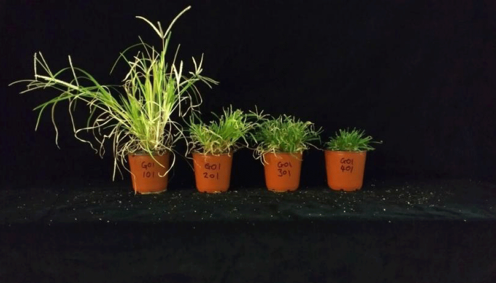
Figure 1: Phenotypes of unmowed goosegrass observed at the completion of the life cycle (~10 weeks) grown under greenhouse conditions at Clemson University, Clemson, SC. The pot (101) to the far left was a wild, upright growing habit, the second pot (201) from the left has an intermediate growth habit (int_I), and the third pot (301) from the left has an intermediate growth habit (int_II), while the far right pot (401) has a dwarf growth habit.
Phenotypic - principle components analysis
To visualize the entire data set and to understand how the measured traits affect the phenotype of various ecotypes, principle components analysis and clustering was performed [4]. The first principal component (PC1) explained 74.7% of the total variation, with highest contributors being height, internode length, raceme length, total biomass and total surface area. The second principal component (PC2), seed head number, explained 16.7% of the total variation (Figure 2). Saidi, et al. [4] noted the main morphological traits for grouping goosegrass ecotypes in Malaysia were number of tillers, flag leaf length, flag leaf width and panicle length. In the present study, the principle components analysis resulted in clustering of individuals within distinct ecotype groups. The dwarf ecotype group clustered between -2 to -3 on PC1, and between -0.8 and -1.2 on PC2 (Figure 2). The int_I ecotype group clustered between 0.2 and -0.8 on PC1, and between 0.8 and -0.5 on PC2 (Figure 2). The int_II ecotype group clustered between -1 and -1.8 on PC1, and between 2.6 and -0.5 on PC2 (Figure 2). The wild ecotype group clustered between 4.8 and 2 on PC1, and between 0 and -0.8 on PC2 (Figure 2). Saidi, et al., noted the number of tillers was a major outlier for Malaysian goosegrass ecotypes [4]. The groupings resulting from the principle components analysis highlight the distinct differences between the four ecotypes based on the morphological traits measured. The ecotypes have been observed in the field for a long time in the southeastern United States. However, this is the first-time distinct groupings of goosegrass ecotypes from the southeastern United States has been achieved through principle components analysis.
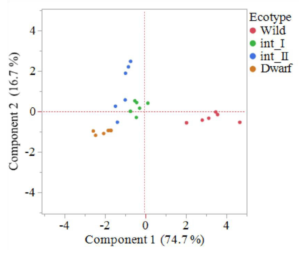
Figure 2: Principle components analysis indicating the grouping of four goosegrass ecotypes; dwarf, intermediate one (int_I), intermediate two (int_II) and wild. Component 1 is a combination of plant height, internode length, raceme length, above ground biomass and total surface area of above ground biomass; component 2 consists of seedhead number. The dwarf ecotype is the lowest on component 1, int_I and int_II are in the middle; and wild is the highest. The int_II ecotype is the highest on component 2; dwarf, int_I and wild are in the middle. Goosegrass plants were grown in greenhouse conditions at Clemson University, Clemson SC. At the completion of the life cycle (~10 weeks) phenotypic data was collected.
Gene sequencing and genetic analysis
In each of the 24 individuals, two genes were sequenced to investigate if the different ecotypes were genetically distinct. Multiple sequence alignment (MSA) of representative samples from the four phenotypically distinct ecotypes revealed genetic variation in the form of single nucleotide polymorphisms (SNP). The orthologous genes in Oryza are as follows: gene A (AP014964) is an expressed eukaryotic protein of unknown function [25] and gene B (AP014965) is a cellulose synthase [26] (Table 1). The two genes were selected as both are under neutral selection pressure. The single consensus phylogenetic tree of gene A and B resulted in distinct clustering of the wild ecotypes (Figure 3). The int_I, int_II and dwarf ecotypes did not result in distinct clustering among the ecotypes (Figure 3). The authors hypothesize that the int_I, int_II and dwarf ecotypes have diverged from the wild ecotypes. The phylogenetic tree constructed would suggest this is the case for the ecotypes in the present study.
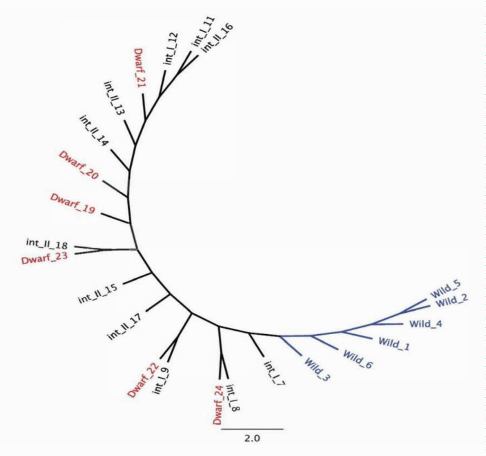
Figure 3: Single consensus phylogenetic tree and associated clustering following multiple sequence alignment of gene A and B; 4 ecotypes include, 6 wild individuals, 5 intermediate one (int_I) individuals, 6 intermediate two (int_II) individuals and 6 dwarf individuals.
Saidi, et al. noted differences in morphology and genetics of goosegrass ecotypes in Malaysia, however, weak correlation occurred between the morphological and molecular data [4]. Weak correlations between morphology and molecular data have also been noted in other plant species such as barley (Hordeum vulgare L.) [27], he guo mu (Paramichelia baillonii Pierre Hu) [28] and potato (Solanum tuberosum L.) [29]. To the authors’ knowledge, this is the first reported case of morphological and genetic differences between goosegrass ecotypes found in the southeastern United States.
Future research is needed to fully understand the genetic and phenotypic relationship between goosegrass ecotypes. Genetic screening of a larger population of ecotypes at multiple loci is needed to understand the complexity and diversity of the goosegrass genome. The current study highlights the need for genotyping by sequencing of the different goosegrass ecotypes. The genotyping by sequencing would result in a more detailed resolution of the goosegrass genome. Further implications could lead to a greater understanding of herbicide resistance mechanisms and highlight potential SNP of weedy traits for breeding programs. The genes used in the present study could be utilized in other plant species to discriminate between ecotypes.
- Agrawal AA. Phenotypic plasticity in the interactions and evolution of species. Science. 2001; 294: 321-326. PubMed: https://www.ncbi.nlm.nih.gov/pubmed/11598291
- Sultan SE. Phenotypic plasticity and plant adaptation. Acta Bot Neerl. 1995; 44: 363-383.
- Geng YP, Pan XY, Xu CY, Zhang WJ, Li B, et al. Phenotypic plasticity rather than locally adapted ecotypes allows the invasive alligatorweed to colonize a wide range of habitats. Biological Invasions. 2007; 9: 245-256.
- Saidi N, Kadir J, Hong LW. Genetic diversity and morphological variations of goosegrass [Eleusine indica (L.) Gaertn] ecotypes in Malaysia. Weed & Turfgrass Sci. 2016; 5: 144-154.
- Chen J, Huang Z, Huang H, Wei S, Liu Y, et al. Selection of relatively exact reference genes for gene expression studies in goosegrass (Eleusine indica) under herbicide stress. Scientific Reports. 2017; 7: 46494.
- Ganeshaiah KN, Shaanker RU. Evolution of reproductive behavior in the genus Eleusine. Euphytica. 1982; 31: 397-404.
- Brosnan JT, Breeden GK. Herbicide resistance in turfgrass: an emerging problem? Outlooks on Pest Manag. 2013; 24: 164-168.
- Lee LJ, Ngim J. A first report of glyphosate?resistant goosegrass (Eleusine indica (L.) Gaertn) in Malaysia. Pest Manag Sci. 2000; 56: 336-339.
- Buker RS, Steed ST, Stall WM. Confirmation and control of a paraquat-tolerant goosegrass (Eleusine indica) biotype. Weed Technol. 2002; 16: 309-313.
- Brosnan JT, Nishimoto RK, de Frank J. Metribuzin-resistant goosegrass (Eleusine indica) in bermudagrass turf. Weed Technol. 2008; 22: 675-678.
- Seng CT, Van Lun L, San CT, Sahid IB. Initial report of glufosinate and paraquat multiple resistance that evolved in a biotype of goosegrass (Eleusine indica) in Malaysia. Weed Biol and Manag. 2010; 10: 229-233.
- McElroy JS, Head WB, Wehtje GR, Spak D. Identification of goosegrass (Eleusine indica) biotypes resistant to preemergence-applied oxadiazon. Weed Technol. 2017; 31: 675-681
- Busey P. Goosegrass (Eleusine indica) control with foramsulfuron in bermudagrass (Cynodon spp.) turf. Weed Technol. 2004; 18: 634-640.
- McCarty LB. Goosegrass (Eleusine indica) control in bermudagrass (Cynodon spp.) turf by diclofop. Weed Sci. 1991; 39: 255-261.
- Burdon JJ. Diseases and Plant Population Biology. Cambridge University Press, Cambridge, UK, 1987.
- Cross RB, McCarty LB, McElroy JS, Tharayil N, Bridges WC. Comparison of enzyme and growth characteristics in ALS-inhibitor susceptible and resistant annual bluegrass (Poa annua) biotypes. Weed Sci. 2015; 63: 220-228.
- Dekker J. Weed diversity and weed management. Weed Sci. 1997; 357-363.
- Varma V, Osuri AM. Black spot: A platform for automated and rapid estimation of leaf area from scanned images. Plant Ecol. 2013; 214: 1529-1534.
- Kubisiak TL, Nelson CD, Staton ME, Zhebentyayeva T, Smith C, et al. A transcriptome-based genetic map of Chinese chestnut (Castanea mollissima) and identification of regions of segmental homology with peach (Prunus persica). Tree Genetics & Genomes. 2013; 9: 557-571.
- Altschul SF, Gish W, Miller W, Myers EW, Lipman DJ. Basic local alignment search tool. J Mol Biol. 1990; 215: 403-410. PubMed: https://www.ncbi.nlm.nih.gov/pubmed/2231712
- Kanapeckas KL, Vigueira CC, Ortiz A, Gettler KA, Burgos NR, et al. Escape to ferality: the endoferal origin of weedy rice from crop rice through de-domestication. PLoS One. 2016; 11: e0162676. PubMed: https://www.ncbi.nlm.nih.gov/pmc/articles/PMC5035073/
- Chen S, McElroy JS, Dane F, Peatman E. Optimizing transcriptome assemblies for Eleusine indica leaf and seedling by combining multiple assemblies from three de novo assemblers. Plant Genome. 2015; 8: 1-10.
- Tanskanen M, Peuralinna T, Polvikoski T, Notkola IL, Sulkava R, et al. Senile systemic amyloidosis affects 25% of the very aged and associates with genetic variation in alpha2?macroglobulin and tau: a population? based autopsy study. Ann Med. 2008; 40: 232-239. PubMed: https://www.ncbi.nlm.nih.gov/pubmed/18382889
- Garcia NS, Sexton J, Riggins T, Brown J, Lomas MW, et al. High variability in cellular stoichiometry of carbon, nitrogen, and phosphorus within classes of marine eukaryotic phytoplankton under sufficient nutrient conditions. Frontiers in Microbiology. 2018; 27: 543. PubMed: https://www.ncbi.nlm.nih.gov/pmc/articles/PMC5880891/
- Wilkins O, Hafemiester C, Plessis A, Holloway-Phillips MM, Pham GM, et al. Environmental gene regulatory influence networks in rice (Oryza sativa): response to water deficit, high temperature and agricultural environments. BioRxiv. 2016; 1: 042317.
- Chandran AK, Jeong HY, Jung KH, Lee C. Development of functional modules based on co-expression patterns for cell-wall biosynthesis related genes in rice. J Plant Biol. 2016; 59: 1-5.
- Lund B. Repatriation of Nordic barley germplasm. Ph.D Dissertation. Copenhagen, Denmark: The Royal Veterinary and Agricultural University. 2002.
- Li F, Gan S, Weng Q, Zhao X, Huang S, et al. RAPD and morphological diversity among four populations of the tropical tree species Paramichelia baillonii (Pierre) Hu in China. Forest Ecology and Manag. 2008; 255: 1793-801.
- Vetelainen M, Gammelgard E, Valkonen JP. Diversity of Nordic landrace potatoes (Solanum tuberosum L.) revealed by AFLPs and morphological characters. Genetic Resources and Crop Evolution. 2005; 52: 999-1010.